Look How Far We’ve Come

Oxford’s Max Roser has provided a much-needed ray of sunshine given the past week’s events. Roser writes,

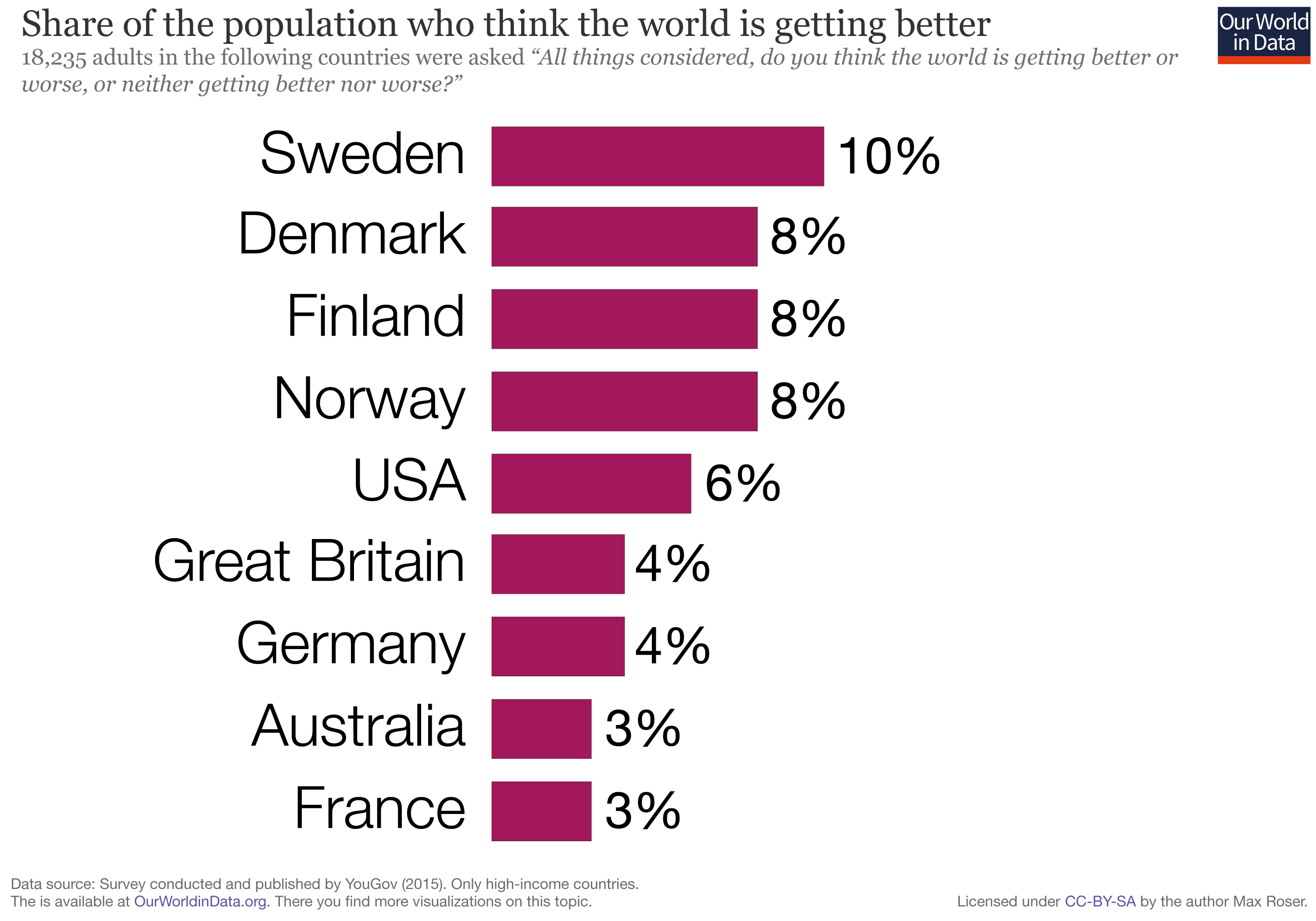
A recent survey asked “All things considered, do you think the world is getting better or worse, or neither getting better nor worse?”. In Sweden 10% thought things are getting better, in the US they were only 6%, and in Germany only 4%. Very few people think that the world is getting better.

What is the evidence that we need to consider when answering this question? The question is about how the world has changed and so we must take a historical perspective. And the question is about the world as a whole and the answer must therefore consider everybody. The answer must consider the history of global living conditions – a history of everyone.

Roser tackles several issues, but I’ve selected just four:

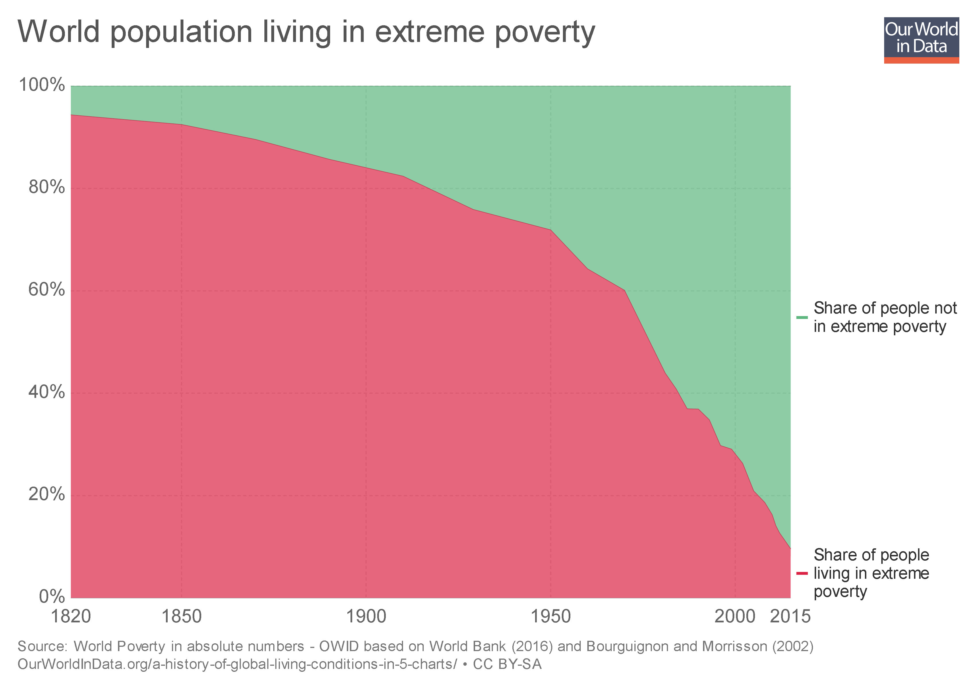
  • Poverty: “Take a longer perspective and it becomes very clear that the world is not static at all. The countries that are rich today were very poor just very recently and were in fact worse off than the poor countries today. To avoid portraying the world in a static way – the North always much richer than the South – we have to start 200 years ago before the time when living conditions really changed dramatically…The first chart shows the estimates for the share of the world population living in extreme poverty. In 1820 only a tiny elite enjoyed higher standards of living, while the vast majority of people lived in conditions that we would call extreme poverty today. Since then the share of extremely poor people fell continuously. More and more world regions industrialised and thereby increased productivity which made it possible to lift more people out of poverty: In 1950 three-quarters of the world were living in extreme poverty; in 1981 it was still 44%. For last year research suggests that the share in extreme poverty has fallen below 10%.”

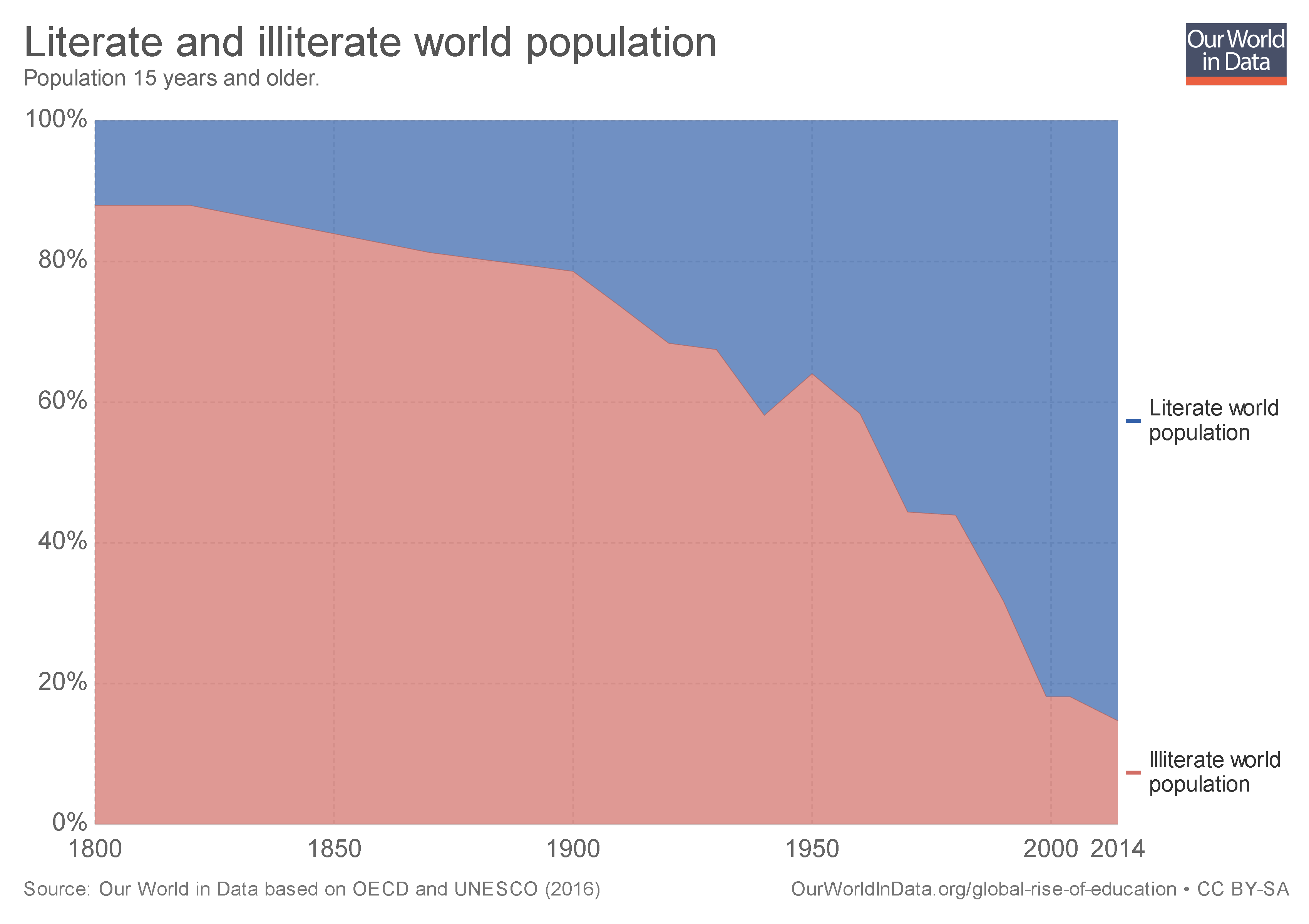
  • Literacy: “How did the education of the world population change over this period? The chart below shows the share of the world population that is literate over the last 2 centuries. In the past only a tiny elite was able to read and write. Today’s education – including in today’s richest countries – is again a very recent achievement. It was in the last two centuries that literacy became the norm for the entire population.”

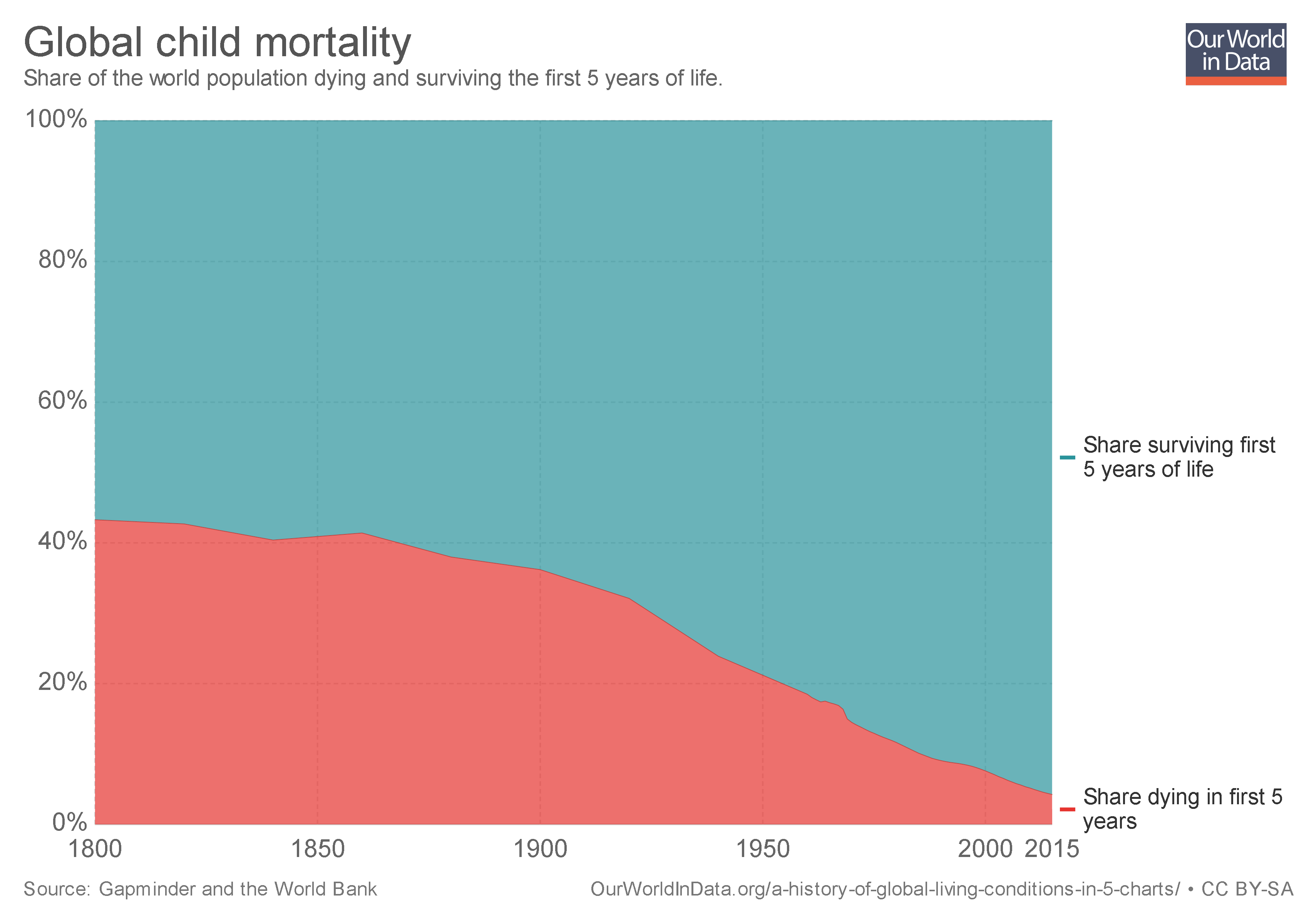
  • Health: “In 1800 the health conditions of our ancestors were such that around 43% of the world’s newborns died before their 5th birthday. The historical estimates suggest that the entire world lived in poor conditions; there was relatively little variation between different regions, in all countries of the world more than every third child died before it was 5 years old…In 2015 child mortality was down to 4.3% – 10-fold lower than 2 centuries ago. You have to take this long perspective to see the progress that we have achieved.”

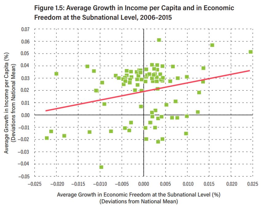
  • Freedom: “Political freedom and civil liberties are at the very heart of development – as they are both a means for development and an end of development…The chart shows the share of people living under different types of political regimes over the last 2 centuries. Throughout the 19th century more than a third of the population lived in colonial regimes and almost everyone else lived in autocratically ruled countries. The first expansion of political freedom from the late 19th century onward was crushed by the rise of authoritarian regimes that in many countries took their place in the time leading up to the Second World War. In the second half of the 20th century the world has changed significantly: Colonial empires ended, and more and more countries turned democratic: The share of the world population living in democracies increased continuously – particularly important was the breakdown of the Soviet Union which allowed more countries to democratise. Now more than every second person in the world lives in a democracy. The huge majority of those living in an autocracy – 4 out of 5 – live in one autocratic country: China. Human rights are similarly difficult to measure consistently over time and across time. The best empirical datashow that after a time of stagnation human right protection improved globally over the last 3 decades.”

Roser concludes,

For our history to be a source of encouragement we have to know our history. The story that we tell ourselves about our history and our time matters. Because our hopes and efforts for building a better future are inextricably linked to our perception of the past it is important to understand and communicate the global development up to now. A positive lookout on the efforts of ourselves and our fellow humans is a vital condition to the fruitfulness of our endeavors. Knowing that we have come a long way in improving living conditions and the notion that our work is worthwhile is to us all what self-respect is to individuals. It is a necessary condition for self-improvement.

Freedom is impossible without faith in free people. And if we are not aware of our history and falsely believe the opposite of what is true we risk losing faith in each other.

Image result for look around at how lucky we are to be alive gif

Are STEM Fields Discriminatory Toward Women?

Image result for negative ghost rider

At least according to a 2015 study:

Our experimental findings do not support omnipresent societal messages regarding the current inhospitability of the STEM professoriate for women at the point of applying for assistant professorships (4122629). Efforts to combat formerly widespread sexism in hiring appear to have succeeded. After decades of overt and covert discrimination against women in academic hiring, our results indicate a surprisingly welcoming atmosphere today for female job candidates in STEM disciplines, by faculty of both genders, across natural and social sciences in both math-intensive and non–math-intensive fields, and across fields already well-represented by women (psychology, biology) and those still poorly represented (economics, engineering). Women struggling with the quandary of how to remain in the academy but still have extended leave time with new children, and debating having children in graduate school versus waiting until tenure, may be heartened to learn that female candidates depicted as taking 1-y parental leaves in our study were ranked higher by predominantly male voting faculties than identically qualified mothers who did not take leaves.

Our data suggest it is an auspicious time to be a talented woman launching a STEM tenure-track academic career, contrary to findings from earlier investigations alleging bias (313), none of which examined faculty hiring bias against female applicants in the disciplines in which women are underrepresented. Our research suggests that the mechanism resulting in women’s underrepresentation today may lie more on the supply side, in women’s decisions not to apply, than on the demand side, in antifemale bias in hiring. The perception that STEM fields continue to be inhospitable male bastions can become self-reinforcing by discouraging female applicants (2629), thus contributing to continued underrepresentation, which in turn may obscure underlying attitudinal changes. Of course, faculty members may be eager to hire women, but they and their institutions may be inhospitable to women once hired. However, elsewhere we have found that female STEM professors’ level of job satisfaction is comparable to males’, with 87%-plus of both genders rating themselves “somewhat to very” satisfied in 2010 (figure 19 in ref. 14). Also, it is worth noting that female advantages come at a cost to men, who may be disadvantaged when competing against equally qualified women. Our society has emphasized increasing women’s representation in science, and many faculty members have internalized this goal. The moral implications of women’s hiring advantages are outside the scope of this article, but clearly deserve consideration.

Real-world data ratify our conclusion about female hiring advantage. Research on actual hiring shows female Ph.D.s are disproportionately less likely to apply for tenure-track positions, but if they do apply, they are more likely to be hired (163034), sometimes by a 2:1 ratio (31). These findings of female hiring advantage were especially salient in a National Research Council report on actual hiring in six fields, five of which are mathematically intensive, at 89 doctoral-granting universities (encompassing more than 1,800 faculty hires): “once tenure-track females apply to a position, departments are on average inviting more females to interview than would be expected if gender were not a factor” (ref. 16, p. 49). [See SI Appendix for descriptions of other audits of actual hiring that accord with this view, some dating back to the 1980s. Many studies have argued (see ref. 14) that because only the very top women persist in math-intensive fields, their advantage in being hired is justified because they are more competent than the average male applicant. This is why an accurate evaluation of gender preference in hiring depends on data from an experiment in which competence is held constant.] Thus, real-world hiring data showing a preference for women, inherently confounded and open to multiple interpretations because of lack of controls on applicant quality, experience, and lifestyle, are consistent with our experimental findings.

Does Collective Bargaining Lead to More Police Misconduct?

Image result for footloose police

That seems to be the case, according to a new study. The researchers explain,

There has been significant scholarly attention recently to the issue of excessive law enforcement violence (Fryer 2016; Legewie and Fagan 2016; Shjarback 2015; Shane, Lawton, and Swenson 2017; Stickle 2016), some of which has trained on the role of collective bargaining (Huq and McAdams 2016; Rushin 2017). No previous work, however, has offered empirical evidence of the causal role that unionization or collective bargaining play in the performance of law enforcement. We offer such evidence by exploiting a January 2003 change in Florida labor law. By a judicial decision that month (Williams), county sheriffs’ deputies won for the first time the right to organize for collective bargaining. Before and after that date, municipal police officers had the right to engage in collective bargaining. We examine how Williams affected complaints of misconduct against law enforcement personnel at these two types of agencies.

Our analysis uses a dataset on Florida law enforcement agencies – covering both county sheriffs’ offices (SOs) and city police departments (PDs) – that begins in 1997 (our primary tests use data for 1997-2010). This dataset combines annual Criminal Justice Agency Profile (CJAP) surveys conducted by the Florida Department of Law Enforcement (FDLE) with administrative data from the FDLE on law enforcement officers and on complaints and disciplinary actions against officers. We analyze in particular the number of complaints at the agency-year level against officers affiliated with each agency. Our empirical strategy involves the use of a difference-indifference framework, in which the treatment group consists of SOs (that were affected by Williams) and the control group consists of PDs (that were unaffected). Officers assigned to agencies in the treatment and control groups perform similar job functions (Pynes and Corley 2006, p. 299). Likewise, similar pools of applicants seek employment with SOs and PDs, and there is lateral movement by officers between the agency types (Baker 2017a).

We begin by showing that Williams led to substantial unionization among SOs. This occurred over a three-year period following the decision, and then stabilized; thus, our primary specifications use a three-year lag of the variable of interest (an interaction between the post-2003 years and an indicator for SOs). Our baseline analysis uses a Poisson maximum-likelihood model in order to accommodate count data on complaints. We control for agency and year fixed effects and for an extensive set of controls (including demographic variables, local economic conditions, and local crime rates). The central result is that collective bargaining rights led to about a 27% increase in complaints of officer misconduct for a typical SO. We also find some evidence that, for agency-years with positive numbers of complaints, the number of state disciplinary actions against officers also increased. We argue in Section 5 below that this suggests that the increased complaints against SOs were not accompanied by a decrease in the seriousness of these complaints.

When adding an extensive set of leads and lags to the basic model, we find that the difference-in-difference estimate is small and statistically insignificant for “false experiments” (or placebo tests) in years prior to 2003, suggesting that the results are not attributable to a preexisting trend toward more complaints against SOs. In a linear framework, the result is robust to adding linear agency-specific time trends and county-by-year fixed effects. Taken together, the results on prior years and on agency-specific time trends suggest that the parallel trend assumption that is crucial in the difference-in-difference framework is satisfied here. This supports a causal interpretation of our findings on the impact of collective bargaining rights, despite numerous factors we describe below that create a bias against our results (pgs. 2-3).

I’m thinking that collective bargaining’s track record isn’t the hottest.

The Long-Term Benefits of Marriage: UK Edition

According to a post at the Institute for Family Studies,

One of the most common critiques of the supposed advantages of marriage is that married adults and their children only do better because of their education and money. The argument goes something like this: “It’s not marriage that conveys the advantages of life. It’s just that those who are better educated are more likely to get married. They then go on to make a success of their family and avoid many of the pitfalls. It’s a ‘mistake’ to attribute this to marriage, when really it’s all about education and money.”

But the actual data say quite the opposite:

Compare rich families or poor families and the outcome tends to be the same. Married families still tend—on average, remember—to do better. We’ve shown this to be the case in a whole range of studies…Anyway, one of my research colleagues—Professor Spencer James at Brigham Young University—and I decided we wanted to look at whether having married parents, rather than unmarried parents, has any long-term effect on life as an adult. We’ve already established that married couples are more likely to stay together. We’ve already established that the children of married adults are more likely to avoid things like mental health problems. In both cases, this is true regardless of parent’s age, education, and ethnicity. 

But how long do these effects last?

To find out, we took a look at two British cohort studies that have followed the lives of 20,000 babies born in 1958 and 1970 who are all now adults in their late 40s and 50s. The timings are different for each cohort, but essentially these adults were asked all sorts of questions every five to 10 years.

This allowed us to compare those born to married and unmarried parents and also look at the social class of the parents when they were aged 16. We then looked at the children who later on got married, those who went to university, and those who needed to make use of benefits at any stage during adulthood to date.

Just to make sure we were looking at any effect of marriage, we also controlled for the child’s sex, mother’s age at birth, and mother’s interest in their child’s education at age 16, and any differences in outcomes between the two surveys.

The results of our study, which is now downloadable from the Marriage Foundation website, were extraordinary. Regardless of family and social background, those born to married parents were:

  • 23% more likely to have been to university

  • 10% more likely to have got married, and

  • 16% less likely ever to have received government benefits

One particularly interesting finding: “Having richer parents made no difference in the probability of ever needing to go on welfare if those parents weren’t initially married. In other words, kids brought up in better-off homes are more likely to go to university and more likely to get married. But if the parents weren’t married, rich kids are just as likely to end up on government benefits as poor kids. There is no effect of money.” The authors suggest,

Even in families where one or both parents are university educated or white-collar workers, children will have seen the difficulty of managing the dissolution of family life. Even among well-educated parents, that might have included a stint on welfare benefits. Having seen that happen to their parents may then reduce the resistance to relying on the government. It may also be that a more relaxed attitude among some lone parents leads to a more relaxed attitude to going on benefits.

Regardless of the explanation, our findings are robust and striking and show at least one major area of life where having married parents has a big impact on the future lives of children, yet money appears to play no role whatsoever.


Formula(s) for Success

How does one become an elite performer or successful at work? According to the Greater Good Science Center,

Angela Duckworth, the celebrated psychologist who first defined “grit” as perseverance and passion for long-term goals, has a theory about success. Instead of seeing achievement as simply a byproduct of IQ or intelligence or innate talent, Duckworth sees achievement as the product of skill and effort (Achievement = Skill x Effort) in the same way that we understand that Distance = Speed x Time.

…Tremendous effort can compensate for modest skill, just as tremendous skill can compensate for modest effort, but not if either is zero.  Researchers across diverse fields have produced remarkably consistent findings that back up Duckworth’s theory. They find that innate ability has relatively little to do with why people go from being merely good at something to being truly great.

This is hard for most of us to believe, but K. Anders Ericsson, a psychologist and author of several landmark studies on this topic, has shown that even most physical advantages (like athletes who have larger hearts or more fast-twitch muscle fibers or more flexible joints—the things that seem the most undeniably genetic) are, in fact, the result of certain types of effort…Even super-skills, like “perfect pitch” in eminent musicians, have been shown to stem from training more than inborn talent. Hard to believe, but entirely true.

…People who rise to greatness tend to have three things in common: 1) They both practice and rest deliberately over time; 2) Their practice is fueled by passion and intrinsic interest; and 3) They wrestle adversity into success.

Elite performers “spend hours upon hours in “deliberate practice.” This isn’t just poking around on the piano because it is fun; it is consistently practicing to reach specific objectives—say, to be able to play a new piece that is just beyond their reach. In the beginning, they may practice a new phrase or even a single measure again and again and again. Unfortunately, deliberate practice isn’t always pleasurable—far from it. In fact, it is the elite performer’s willingness to engage in hard or, quite often, very boring, practice that distinguishes people who are good at their chosen activity from those who are the very best at it.” They “also practice consistently over a pretty long period of time.”

Image result for violin gif your lie in aprilProper rest is also extremely important. “In his studies of truly great performers, K. Anders Ericsson, the psychologist and author of several landmark studies on elite performance…found that they practiced and rested a lot more than their good but not elite peers. For example, violinists destined to become professional soloists practiced an average of 3.5 hours per day, typically in three separate sessions of 60-90 minutes each. Good but not great performers, in contrast, typically practiced an average of 1.4 hours per day, with no deliberate rest breaking up their practice session…The top violins [also] slept an hour a night more than their less-accomplished classmates. They were also far more likely to take a nap between practice sessions—nearly three hours of napping a week.” It turns out that top achievers “sleep significantly more than the average American. On average, Americans get only 6.5 hours of sleep per night. (Even though studies show that 95 percent of the population needs between seven and eight hours of sleep a night.) Elite performers tend to get 8.6 hours of sleep a night; elite athletes need even more sleep. One study showed that when Stanford swimmers increased their sleep time to 10 hours a night, they felt happier, more energetic—and their performance in the pool improved dramatically.”

Failure is also a part of success. “Elite performers turn adversity into success. Most greats don’t just pile up one achievement after the next. Failure is a key part of growth and, eventually, elite performance”:

Failure—and adversity in general—is life’s great teacher. While there might not be anything good in misfortune, as Viktor Frankl wisely reminds us, it is often possible to wrench something good out of misfortune. We know that adverse life-events—a plane crash, a terrorist bombing, breast cancer—can trigger depression, anxiety, and posttraumatic stress syndrome. But what most of us don’t realize is that posttraumatic growth, as researchers call it, can also awaken us to new strength and wisdom. Misfortune—even tragedy—has the potential to give our lives new meaning and a new sense of purpose, and in this way, adversity also contributes to the passion part of the grit equation.

Finally, a five-year study of nearly 5,000 managers and employees in the U.S. finds five major strategies for work success and well-being:

  • intensely focusing on few tasks.”
  • “prioritize work that [you] can do well, efficiently, and with great benefit to others.”
  • “engage in collaboration only when it ma[kes] good business sense and when working together [i]s a benefit rather than a hassle.”
  • “success requires the support of others, and the best way to garner that support is to speak to people’s values, interests, and motivations.”
  • combine passion “with a sense of purpose.”

Try testing out these formulas in your own life.

Will Inexpensive Health Insurance Lead to Full Coverage?

According to data from Massachusetts’ Commonwealth Care program, “even if 90 percent of health insurance costs were subsidized, 25 percent of those eligible for subsidies would choose to remain uninsured.” The program

offers large subsidies for private health insurance for individuals below 300 percent of the federal poverty level who are not covered by an employer plan or another public program, such as Medicare. The researchers analyze data from fiscal year 2011. Insurance payments were covered by a combination of Commonwealth Care subsidies and premiums paid by the eligible individuals. Enrollee premiums, intended to be affordable for low-income people, varied with income levels. Specifically, rate changes occurred at 150 percent, 200 percent, and 250 percent of the poverty line. The premium for the cheapest plan was $39 a month for enrollees with incomes between 150 and 200 percent of the poverty line, $77 a month for those from 200 to 250 percent, and $116 a month for those above 250 percent. All of these enrollee premiums were heavily subsidized relative to insurers’ costs, which averaged $359 per month. Individuals could choose to forgo coverage and pay a penalty equal to half the cost of the lowest premium.

The variation in the post-subsidy cost of insurance for low-income participants allows the researchers to estimate enrollees’ willingness to pay for health insurance. It also enables them to study how the set of enrollees who take up insurance affects provider costs. The researchers find that for each $40 increase in monthly premiums for the cheapest plan, enrollment in Commonwealth Care declined by about 25 percent, despite the penalty for opting out of coverage. When Commonwealth Care was free — as it was for those below 150 percent of the poverty line — 94 percent of eligible adults enrolled, but participation decreased to 70 percent when the premium rose to $39 per month, and to below 50 percent when premiums were $116 per month.

As individuals dropped out of coverage when their premiums became more expensive, average insurer costs per participant rose. At the 150 percent threshold, insurer costs increased by $47 per enrollee, or 14 percent. This indicates that the individuals who dropped coverage as the price increased were, on average, less expensive individuals to insure. In other words, the insured pool was adversely selected in terms of health risk.

The researchers estimate that individuals are willing to pay less than one-third of average insurer costs to obtain coverage. The median willingness to pay for insurance is $100 a month, roughly one-fourth of the cost of insuring individuals with above-median willingness to pay. Thus if a subsidy covers 75 percent of the cost of coverage, only half of eligible participants would choose to buy insurance. Even if the subsidy were 90 percent, 25 percent of those eligible would choose to remain uninsured.

Read the full working paper here.

Was the China Shock Actually a Boom?

I’ve talked about the China Shock before. The concern is that imports from China reduced the amount of jobs in the United States. However, new research suggests otherwise:

Our empirical results show important job gains due to US export expansion. We find that although imports from China reduce jobs, the global export expansion of US products creates a considerable number of jobs. Based on the industry-level estimation, our results show that on balance over the entire 1991-2007 or 1991-2011 periods, job gains due to changes in US global exports largely offset job losses due to China’s imports, resulting in about 300,000 to 400,000 job losses in net. Estimation at the commuting zone level generate even bigger job creation effects: in net, global export expansion substantially offsets the job losses due to imports from China, resulting in about 200,000 net job losses over the period 1991-2007, and a roughly balanced net effect if we extend the analysis to 1991-2011.

In Feenstra and Sasahara (2017), we quantify the employment effect of US imports and exports using a global input-output analysis. Following the technique of Los et al. (2015), we use the world input-output table from WIOD and examine the employment effects of US total exports and imports from China and from all countries during the period 1995-2011. Admittedly, this approach only indicates the impact of trade on labour demand, without taking into account the (regional) supply of labour in general equilibrium.

We find that the growth in US exports created demand for 2 million manufacturing jobs, 500,000 resource-sector jobs, and a remarkable 4.1 million jobs in services, totalling 6.6 million. The positive job creation effect of exports in the manufacturing sector, 2 million, is quantitatively similar to the result in Feenstra et al. (2017), in which 1.9 million jobs were created by US exports from the instrumental-variable regression approach. On the import side, our analysis shows that manufacturing imports from China reduced demand for US jobs by 1.8-2.0 million, which is similar to the result in Autor et al. (2016), who finds a decline of 2.0 million jobs due to imports from China.

One advantage of the input-output approach is that it is easy to extend the analysis to other sectors such as services and natural resources. Our results show that, when focusing on the manufacturing sector and the natural resource sector, the net effect of overall trade with all countries in all sectors is slightly negative: 80,000 reduction in demand for jobs in manufacturing, and a 250,000 job reduction in the natural resource sector during 1995-2011. However, when looking at the service sector, we find a substantial net job gain, with a 1.03 million increase in the demand for jobs due to overall trade with all countries. This is large enough to compensate for the net job losses in the manufacturing and natural resource sectors. After taking all of these into account, the net effect of overall trade with all countries led to a net increase in labour demand of 700,000 jobs.

They conclude,

Our results fit the textbook story that job opportunities in exports make up for jobs lost in import-competing industries, or nearly so. Once we consider the export side, the negative employment effect of trade is much smaller than is implied in the previous literature. Although our analysis finds net job losses in the manufacturing sector for the US, there are remarkable job gains in services, suggesting that international trade has an impact on the labour market according to comparative advantage. The US has comparative advantages in services, so that overall trade led to higher employment through the increased demand for service jobs.


Does More Gender Egalitarianism Reduce Gender Differences?

Image result for we're different gif

Perhaps surprisingly, the answer appears to be “no.” A 2017 study in the International Journal of Psychology found,[ref]Previous studies have come to similar conclusions.[/ref]

Gender differences in most psychological traits—Big Five, Dark Triad, self-esteem, subjective well-being, depression and values—are larger in cultures with more gender egalitarianism. Gendered socialization practices, sociopolitical institutions and gender role stereotypes—some of which appear universal across cultures (Low, 1989; Nosek et al., 2009; Williams & Best, 1990)—undoubtedly influence men’s and women’s personalities to some degree (Kring & Gordon, 1998; Twenge, 1997). Nevertheless, the limited evidence reviewed here casts serious doubts on social role theory’s ability to accurately predict and explain cross-cultural variations in the relative size of psychological gender differences. Simply put, when the men and women of a nation perceive the most similar gender roles, receive the most similar gender role socialization, and experience the greatest sociopolitical gender equity, gender differences in personality are almost always at their largest.

Beyond personality traits, similar disconfirmations of social role theory’s cross-cultural predictions have been demonstrated across a variety of human attributes. For instance, gender differences in romantic attitudes and behaviours—including dismissing attachment, intimate partner violence, love, enjoying casual sex and mate preferences for attractiveness—also appear noticeably larger in cultures with more gender egalitarianism (Schmitt, 2015; for notable exceptions, see Schmitt, 2005; Zentner & Eagly, 2015). Gender differences in many objectively tested cognitive measures—such as spatial location, spatial rotation and episodic memory abilities—also appear larger in cultures with more gender egalitarianism (Silverman, Choi, & Peters, 2007; Weber, Skirbekk, Freund, & Herlitz, 2014). Lippa, Collaer, and Peters (2010) tested spatial rotation abilities in men and women across 40 nations, the largest gender differences in spatial rotation ability were found in Norway, the smallest were found in Pakistan. In a review of gender differences in mathematics test scores within and across cultures, Stoet and Geary (2013) concluded the evidence is mixed, but “If anything, economically developed countries with strong gender-equality and human development scores tended to have a larger sex difference in mathematics” (p. 4). Even gender differences in physical characteristics such as height, obesity and blood pressure are conspicuously larger in cultures with more gender egalitarianism (Schmitt, 2015) (pg. 49).

In short,

the vast weight of the extant evidence suggests the relatively large gender differences observed in Northern European nations are unlikely to be the result of psychological blank slates in boys and girls being written on by especially potent gender role socialization practices or especially strong sociopolitical patriarchy within Scandinavian cultures. Instead, psychological gender differences—in Big Five traits, Dark Triad traits, self-esteem, subjective well-being, depression and values—are demonstrably the largest in cultures with the lowest levels of bifurcated gender role socialization or sociopolitical patriarchy. Ultimately, the view that men and women start from a blank slate simply does not jibe with the current findings, and scholars who continue to assert gender invariably starts from a psychological blank slate should find these recurring cross-cultural patterns challenging to their foundational assumptions (pg. 50).

The researchers conclude,

It is undeniably true that men and women are more similar than different genetically, physically and psychologically. Even so, important gender differences in personality exist that likely stem, at least in part, from evolved psychological adaptations. Some of these adaptations generate culturally-universal gender differences, and many are further designed to be sensitive to local socioecological contexts in ways that facultatively generate varying sizes of gender differences across cultures. It is also true evolved gender differences in personality can be accentuated or attenuated by factors that have little to do with evolved sensitivities to socioecological contexts (Schmitt, 2015). Even gender differences in our bones can embody peculiarities of local cultural forms (Fausto-Sterling, 2005). To shift away from the dominant gender difference paradigm in psychological science—the view that perceived gender roles, gendered socialization and patriarchal sociocultural institutions are the primary causes of psychological gender differentiation (also called the Standard Social Science Model; Tooby & Cosmides,1992)—will no doubt take some time (pg. 52).

Related image

Economic Freedom of North America 2017

The Fraser Institute–who publishes the oft-cited Economic Freedom of the World report–published their latest Economic Freedom of North America report toward the end of December. This report looks at states within Canada, the United States, and Mexico. Once again, there is a link between economic freedom and economic well-being.

I’m happy to report that Texas is tied with Florida for the 2nd most economically free state in the United States and tied for 3rd (along with 10 other U.S. states, including Florida, South Dakota, Nevada, and Georgia) at the national level. Yet, the Cato Institute’s Freedom in the 50 States report finds that we could do better when it comes to personal freedom:

Personal freedom is relatively low in Texas, but it should rise with the Obergefell decision, setting aside Texas’s super-DOMA…Criminal justice policies are generally aggressive—though Texas has emerged as a leading voice in the national reform movement. Even controlling for crime rates, the incarceration rate is far above the national average and has not improved since 2000. Drug arrest rates have fallen over time but are still above average for the user base. Nondrug victimless crime arrest rates have also fallen over time and are now below the national average. Asset forfeiture is mostly unreformed, and law enforcement frequently participates in equitable sharing. Cannabis laws are harsh. A single offense not involving minors can carry a life sentence. Even cultivating a tiny amount carries a mandatory minimum of six months. In 2013–14, the state banned the mostly harmless psychedelic Salvia divinorum. Travel freedom is low. The state takes a fingerprint for driver’s licenses and does not regulate automated license plate readers at all. It has little legal gambling. Private school choice programs are nonexistent, but at least private schools and homeschools are basically unregulated. Tobacco freedom is moderate, as smoking bans have not gone as far as in other states. Gun rights are moderately above average and should improve a bit in the next edition with the new open-carry law. Alcohol freedom is above average, with taxes low. Texas has virtually no campaign finance regulations.

Both are useful indices.

Does College Partying Increase the Number of Rapes?

Image result for college party gif

According to a new study,

There are several mechanisms through which partying may increase the incidence of rape among college students. The most obvious relate to alcohol consumption, which has direct pharmacological effects on aggression and cognitive functioning. Moreover, consistent with Becker’s (1968) seminal model of crime, potential perpetrators may believe that the probability of being punished (and the degree of punishment) will be lower if they and/or their victims are inebriated. That said, partying may also increase the incidence of rape by increasing social contact and by altering the context in which social contact takes place. These potential pathways are supported by statistics indicating that over a half of incapacitated rapes and a quarter of forcible rapes take place at parties (Krebs et al. 2009) and statistics indicating that two-thirds of student rape victims are intoxicated or impaired by drugs at the time of the incident (Kilpatrick et al. 2007). Moreover, 77 percent of students agree that reducing drinking would be very effective, or somewhat effective, in preventing sexual assault on their campus (Washington Post-Kaiser Family Foundation 2015) (pg. 236).

So how do the researchers determine if there is an empirical link? By focusing on

the effects of football games–which intensify partying among college students–on the incidence of rape at schools with Division 1 programs. Specifically, we use panel data from the National Incident Based Reporting System to estimate the increases in reports of rape caused by football games using an identification strategy that exploits plausibly random variation in the timing of game days. Intuitively, we identify the effects by comparing reports of rape to law enforcement agencies serving students on game days to reports on nongame days, while controlling for differences expected across different days of the week and across different times of the year. This approach is similar to that of Rees and Schnepel (2009), who analyze the effects of college football games on assault, vandalism, disorderly conduct, and alcohol-related crimes. We find significant and robust evidence that football game days increase reports of rape victimization among 17–24-year-old women by 28 percent. Home games increase reports by 41 percent on the day of the game and away games increase reports by 15 percent. These effects are greater for schools playing in the more prominent subdivision of Division 1 and for relatively prominent games. There is no evidence that these effects are offset by reductions in nearby areas, on adjacent days, or during other times of the fall term. Moreover, the effects are driven largely by 17–24-year-old offenders and by offenders unknown to the victim, though we also find significant effects on incidents involving offenders of other ages and on incidents involving offenders known to the victim. Estimates by race indicate that the main results are not driven solely by white victims or black victims, nor by white offenders or black offenders.

Back of the envelope calculations based on our estimates imply that the effects of Division 1A football games explain 5 percent of fall semester (September through December) reports of rape involving 17–24-year-old victims to law enforcement agencies serving students attending these schools. Moreover, they imply that these games cause 724 additional rapes per year across the 128 schools participating in Division 1A. Based on an estimated social cost of $267,000 per rape (McCollister, French, and Fang 2010), this implies an annual social cost of rapes caused by Division 1A games of $193 million. The estimated effects for schools participating in Division 1AA are smaller, suggesting 108 additional rapes per year across 125 schools (pg. 237).

They also find evidence for “that the effects are larger-than-average for schools that have reputations as “party schools.” Finally, an analysis of the timing of the impacts reveals significant effects on reports of rape the night before, during, and after home games whereas effects are only apparent after away games. This evidence is consistent with there being an effect of pregame partying, which we would expect to be much more common for home than away games” (pg. 238).

A case where empirical evidence backs intuition.