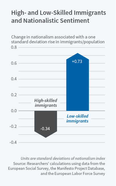
In Skill of Immigrants and Vote of the Natives: Immigration and Nationalism in European Elections 2007-16 (NBER Working Paper No. 25077), Simone Moriconi, Giovanni Peri, and Riccardo Turati explore the relationship between immigration and European elections. They develop an index of “nationalistic” attitudes of political parties to measure the shift in preferences among voters when confronted with influxes of skilled and unskilled immigrants. They find that larger inflows of highly educated immigrants dampen nationalistic sentiments, while larger inflows of less-educated immigrants heighten them. Their results imply that a more balanced inflow of high-skilled and low-skilled immigrants could attenuate voters’ nationalistic attitudes.
...The new study tracks voter attitudes and behavior for all political parties and elections in 12 European countries for a decade. It relies on demographic and political data from the European Social Survey and a number of other sources. In addition, the researchers collected and classified the political manifestos of 126 parties for 28 elections, focusing in particular on how frequently these materials mentioned nationalistic subjects, the European Union, and other indicators of where parties stood on the political spectrum.
The researchers found “that highly educated native voters are less nationalistic in their attitudes towards immigrants than less-educated natives. The data also show strong nationalistic sentiments in regional pockets in the United Kingdom, Ireland, France, Germany, Demark, Sweden, Norway and, especially, Italy.”
The results suggest that a 1 percent increase in the share of a country’s population who are immigrants in highly educated, highly skilled groups was associated with a 0.1 standard deviation voting change away from nationalism. An increase of comparable size in the number of less-educated and lower-skilled immigrants led to a 0.12 standard deviation voting change towards nationalism. The same patterns emerged when the researchers analyzed voter sentiment expressed in surveys. In this case, a 1 percent increase in high-skilled immigrants led to a 0.07 standard deviation decrease away from nationalism, while a 1 percent increase in lower-skilled immigrants lead to a 0.07 standard deviation increase in nationalism. The results were broadly similar regardless of whether the analysis focused on all immigrants or only on immigrants from non-EU nations.
Immigration is not only about ethnicity, but class as well.
The above comes from Michael Moore’s Sicko. Cuba’s healthcare system is a common talking point among those of Moore’s persuasion. However, a recent study should give us pause regarding some of the overly positive claims about Cuba’s system. First, what people like Moore get right:
How is Cuba healthy while poor? Most attribute the fact to Cuba’s zero monetary cost health care system. There is some truth to that attribution. With 11.1% of GDP dedicated to health care and 0.8% of the population working as physicians, a substantial amount of resources is directed towards reducing infant mortality and increasing longevity. An economy with centralized economic planning by government like that of Cuba can force more resources into an industry than its population might desire in order to achieve improved outcomes in that industry at the expense of other goods and services the population might more highly desire (pg. 755).
However,
Centralized planning has disadvantages. Physicians are given health outcome targets to meet or face penalties. This provides incentives to manipulate data. Take Cuba’s much praised infant mortality rate for example. In most countries, the ratio of the numbers of neonatal deaths and late fetal deaths stay within a certain range of each other as they have many common causes and determinants. One study found that that while the ratio of late fetal deaths to early neonatal deaths in countries with available data stood between 1.04 and 3.03 (Gonzalez, 2015)—a ratio which is representative of Latin American countries as well (Gonzalez and Gilleskie, 2017). Cuba, with a ratio of 6, was a clear outlier. This skewed ratio is evidence that physicians likely reclassified early neonatal deaths as late fetal deaths, thus deflating the infant mortality statistics and propping up life expectancy. Cuban doctors were re-categorizing neonatal deaths as late fetal deaths in order for doctors to meet government targets for infant mortality.
Using the ratios found for other countries, corrections were proposed to the statistics published by the Cuban government: instead of 5.79 per 1000 births, the rate stands between 7.45 and 11.16 per 1000 births. Recalculating life expectancy at birth to account for these corrections (using WHO life tables and assuming that they are accurate depictions of reality), the life expectancy at birth of men by between 0.22 and 0.55 years (Gonzalez, 2015) (pg. 755).
But that’s not the only thing driving low infant mortality rates:
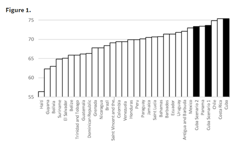
Coercing or pressuring patients into having abortions artificially improve infant mortality by preventing marginally riskier births from occurring help doctors meet their centrally fixed targets. At 72.8 abortions per 100 births, Cuba has one of the highest abortion rates in the world. If only 5% of the abortions are actually pressured abortions meant to keep health statistics up, life expectancy at birth must be lowered by a sizeable amount. If we combine the misreporting of late fetal deaths and pressured abortions, life expectancy would drop by between 1.46 and 1.79 years for men. In Figure 1 below, we show that that with this adjustment alone, instead of being first in the ranking of life expectancy at birth for men in Latin America and the Caribbean, Cuba falls either to the third or fourth place depending on the range (pg. 755-756).
The researchers explain, “Other repressive policies, unrelated to health care, contribute to Cuba’s health outcomes” (pg. 756) These include:
Restrictions in car ownership leading to low automobile fatalities.
Rationing combined with physically demanding transportation (e.g., cycling) contributing to reductions in obesity and deaths caused by diabetes, coronary heart diseases and strokes.
The researchers conclude,
Cuban mortality and longevity statistics appear impressive. They are a result of some combination of the government’s choice to allocate more resources into the health care industry (at the expense of other industries that could produce needed goods) and from coercive measures through both health delivery and economic planning that improve health statistics at the expense of other spheres of life.
Although the USA and other countries re-examine how to design health care delivery they should not uncritically accept the myth that the Cuban health care system has been the sole, or even the most important, cause of Cuba’s abnormally high longevity statistics. The role of Cuban economic and political oppression in coercing ‘good’ health outcomes merits further study (pg. 756).
Walmart catches a lot of grief. For example, as reported by CNN, Bernie Sanders recently “introduced a bill, titled the Stop Walmart Act, that would prevent large companies from buying back stock unless they pay all employees at least $15 an hour, allow workers to earn up to seven days of paid sick leave and limit CEO compensation to no more than 150 times the median pay of all staffers.” Yet, many don’t consider the massive benefits produced by Walmart:
A 2005 Global Insight study commissioned by Wal-Mart and overseen by an independent panel suggested that a new Wal-Mart would create, on net, 137 jobs in the short term and 97 jobs in the long term (Global Insight 2005: 2). Studying Pennsylvania counties, Hicks (2005, discussed by Vedder and Cox 2006: 110) found that the company led to a net increase of fifty new jobs with a 40% reduction in job turnover. Hicks (2007: 93-94) uses data from Indiana to estimate that Wal-Mart increases rural retail employment from 3.4% to 4.8% after correcting for endogeneity. After correcting for endogeneity of urban Wal-Mart entry, Hicks argues that Wal-Mart leads to a 1.2% increase in employment but points out that this estimate is statistically insignificant.
…Wal-Mart’s most obvious effect on the retail sector comes through its policy of Every Day Low Prices. Basker (2005b) and Basker and Noel (2009) estimate that WalMart has a substantial price advantage over competitors with the effect being that prices among incumbent competitors fall after Wal-Mart entry. Hausman and Leibtag (2007: 1147) argue that the compensating variation from Big Box retailers’ effect on prices leads to welfare increases of some 25% of total food expenditure for people who enjoy the direct and indirect effects of Big Box stores. Further, they argue (Hausman and Leibtag 2009) that the Consumer Price Index is over-estimated because it fails to account properly for price effects of supercenters, mass merchandisers, and club stores. Evaluating estimates of the price effects of Big Box retailers and adjusting for foreign sales, Vedder and Cox (2006: 18-19) argue that “the annual American-derived welfare gains are probably still in excess of $65 billion, or about $225 for every American, or $900 for a typical family of four.”
…Jason Furman (2005) called Wal-Mart a “progressive success story” because of its impact on prices. He notes that if the 2005 Global Insight estimate of annual average household savings of $2,329 is accurate, the annual Wal-Mart related consumer savings of $263 billion dwarfs Wal-Mart-generated reductions in retail wages of $4.7 billion estimated by Dube et al. (2005). Hicks (2007: 82) notes that reductions in nominal retail wages are likely offset by larger price reductions, which translates into higher real wages. Courtemanche and Carden’s (2011a) estimate of $177 per household in savings attributable to the effects of Wal-Mart Supercenters in 2002 multiplied by the 105,401,101 households in the 2000 census yields household savings of $18.7 billion, which is still substantially higher than Dube et al.’s estimate of lost wages.
Hausman and Leibtag (2007: 25) argue that the compensating variation—i.e., welfare increase—attributable to supercenters, mass merchandisers, and club stores is some 25% of food expenditures. Since poorer households spend more of their income on food, the effect (as a percentage of income) is higher toward the bottom of the income distribution (Furman 2005: 2-3). Hausman and Leibtag (2007: 1172, 1174) further argue that compensating variation from access to non-traditional retailers is higher at lower income levels, which would make the effect even more progressive (pgs. 8-9).[ref]This doesn’t even address the overseas benefits.[/ref]
A brand new study demonstrates even more benefits provided by Walmart:
We estimate the effects that Walmart Supercenters have on food security using data from the 2001–2012 waves of the December Current Population Study Food Security Supplement (CPS-FSS). Narrow geographic identifiers available in the restricted version of these data enable us to compute the distance from each household’s census tract to the nearest Walmart Supercenter. Our outcomes are counts of the number of affirmative responses on the household and child-specific portions of the food insecurity questionnaire, along with binary variables for household food insecurity, household very low food security, child food insecurity, and child very low food security. We estimate instrumental variables (IV) models that leverage the predictable geographic expansion patterns of Walmart Supercenters outward from corporate headquarters. Specifically, we instrument for Walmart Supercenters with the interaction of distance from Bentonville, Arkansas (Walmart’s headquarters), with time. For both households in general and children specifically, the results show that a closer proximity to the nearest Walmart Supercenter leads to sizeable and statistically significant improvements in all food security measures except the indicator for very low food security. Subsample analyses reveal that the effects are especially large for low-income households and children, though they are also sizeable for middle-income children.
As journalist John Tierney asked, “How could any progressive with a conscience oppose an organization that confers such benefits?”
Drawing on the EFW Index, Brennan (2016a)…points to a strong positive correlation between a country’s degree of economic freedom and its lack of public sector corruption. Granted, a lack of corruption could very well give rise to market reforms and increased economic freedom instead of the other way around. However, recent research on China’s anti-corruption reforms (Ding et al. 2017; Li et al. 2017) suggests that markets may actually pave the way for anti-corruption reforms (pg. 425).
Furthermore,
Market liberalisation can also have indirect effects on war and violence. For example, Neudorfer and Theuerkauf (2014) explore the effects of public sector corruption on ethnic violence by analysing 81 to 121 countries between 1984 and 2007. They find that corruption has a robust positive effect…on the risk of ethnic civil war. When the evidence provided in the previous sections by Brennan (2016a) and Lin et al. (2017) is considered, we find that market liberalisation deters corruption and, consequently, ethnic violence (pg. 429).
Research suggests that economic growth may reduce corruption:
The traditional explanation for this relationship has been the theory articulated by Wolfenson above – corruption increases the cost and risk of business activity, thereby deterring investment and depressing growth that could have lifted citizens out of poverty (Mauro 1995, Wei 1999).
However, there is an alternative possibility that has received less attention among development practitioners and academics. The strong relationship between income and growth may result from exactly the opposite causal relationship – countries may be growing out of corruption (Tresiman 2002). Over time, economic growth reduces both the incentives for government officials to extract bribes and firms’ willingness to pay them. Some scholars of developed countries have discussed this possibility in terms of a ‘life cycle’ theory with corruption peaking at early stages of development and declining as countries industrialise (Huntington 1968, Theobald 1990, Ramirez 2013). However, there has been little work either testing for this empirical link from growth to corruption, or laying out the specific mechanisms that could generate the link.
The authors continue:
The key theoretical insight of our argument is that the share of bribes that officials will choose to extract as rents depends on a firm’s ability to move and set up business in a different location. Ask for too much, and firms that have the ability to do so, will simply pull up anchor and head to safer harbours. Because officials know this, they are likely to set a bribe amount that is just below the cost of moving.
Building on that insight, we show that as firms grow the cost of moving should decline relative to firm size. The fixed cost of moving becomes less expensive relative to revenue, and more and more firms have the opportunity to escape the bribe requests of officials in their locality. Corrupt officials faced with a sudden growth surge must lower their bribe rates, or face losing their key providers of employment and tax payers to competitors.
…The theory we propose has important policy implications. To the extent this theoretical mechanism is important, rather than focusing on politically difficult institutional changes to combat corruption, resources might be better spent on policies that facilitate capital mobility across subnational jurisdictions. Providing clear titles to business premises, for instance, enables entrepreneurs to sell and recoup the full market value of land. Such businesses are more mobile than renters or owners with insecure titles, who risk significant losses if they try to escape corruption by fleeing across the border.
Drawing on “an annual survey funded by USAID and administered by the Vietnamese Chamber of Commerce and Industry,” the researchers find “that the average bribe rate decreases as GDP per capita increases” and “that large firms actually pay lower bribe rates, which is what our theory predicts. Firms with higher revenues are more put out by a high bribe rate, since it increases the amount of bribes they must pay dramatically. To retain them then, officials must push their bribe rate lower.”
Then, using “a census of firms conducted by Vietnam’s General Statistical Office (GSO) [to] calculate aggregate employment at the province-industry-year level,” the authors
show that exogenous industry-wide performance is indeed a strong predictor of a firm’s performance. A doubling of total employment in the industry is associated with a 1.6 percentage point reduction in the bribe rate, or about 42% of the mean level. Moreover, the effect is more pronounced for highly mobile firms. The magnitude of the effect of growth on bribe reductions is 17% larger for firms in possession of a Land Use Rights Certificate, which facilitates the sale of their business premises. Similarly, the effect is 20% greater for firms that already have branch operations in other provinces, and therefore possess knowledge and experience that could facilitate movement.
These effects survive a battery of robustness tests and alternative specifications, providing compelling evidence that growth can directly reduce corruption.
In short, economic growth can decrease corruption by undermining the power of officials to extract bribes. But this is likely part of a virtuous feedback loop. For example, a 2017 paper
exploit[s] spatial variation in randomized anti-corruption audits related to government procurement contracts in Brazil to assess how corruption affects resource allocation, firm performance, and the local economy. After an anti-corruption crackdown, regions experience more entrepreneurship, improved access to finance, and higher levels of economic activity. Using firms involved in corrupt business with the municipality, we find that two channels explain these facts: allocation of resources to less efficient firms, and distortions in government dependent firms. The second channel dominates, as after the audits government dependent firms grow and reallocate resources within the organization (pg. 31).
Of course, it is far easier to demonstrate correlation than causation, and while some studies do find markets playing a causal role in moral development, most simply establish a positive relationship. However, findings that ‘merely’ demonstrate positive correlations should be interpreted in light of the feedback loops: even if moral behaviours are foundational and give rise to market systems (instead of vice versa), market systems in turn reinforce these virtues by imbuing them with value. As Paul Zak (2011, p. 230) explains, ‘Markets are moral in two senses. Moral behavior is necessary for exchange in moderately regulated markets, for example, to reduce cheating without exorbitant transaction costs. In addition, market exchange itself can lead to greater expression of morals in nonmarket settings’ (pg. 423).
Similar to previous research, a new working paper shows that the gender wage gap is driven largely by the amount of hours men and women choose to work. The authors draw on data from the Massachusetts Bay Transportation Authority (MBTA), explaining that the “bus and train operators are all represented by the same union, Carmen’s Local 589, and are all covered by the same bargaining agreement. The agreement specifies that seniority in one’s garage is the sole determinant of one’s work opportunities. Conditional on seniority, men and women face the same choice sets of schedules, routes, vacation days, and overtime hours, among other amenities” (pg. 2).
What do they find?
We show that a gender earnings gap can exist even in a controlled environment where work tasks are similar, wages are identical, and tenure dictates promotions. The gap of $0.89 in our setting, which is 60% of the earnings gap across the United States, can be explained entirely by the fact that, while having the same choice sets in the workplace, women and men make different choices. Women use the Family Medical Leave Act (FMLA) to take more unpaid time off than men and they work fewer overtime hours at 1.5 times the wage rate. At the root of these different choices is the fact that women value time and flexibility more than men. Men and women choose to work similar hours of overtime when it is scheduled a quarter in advance, but men work nearly twice as many overtime hours than women when they are scheduled the day before. Using W-4 filings to ascertain marital status and the presence of dependents, we show that women with dependents – especially single women – value time away from work more than men with dependents.
When selecting their work schedule for the following quarter, women try to avoid inconvenient days, like weekends, and shifts, like split-shifts, more than men. Prioritizing schedule related amenities over route quality-related amenities, women select routes with higher probabilities of assaults and collisions in order to avoid unfavorable schedules. When faced with having to work an unfavorable schedule, like a weekend, holiday, or split shift, women take more unpaid time off. Men also take more unpaid time off in those circumstances, but they more than make up for lost earnings with overtime. While constrained schedules lead to lower earnings for women, they result in higher earnings for men. In an effort to reduce absenteeism and overtime expenditures, the MBTA oversaw two policy changes: one that made it harder to take unpaid time off with FMLA and another that made it harder to be paid at the overtime rate. While the policy changes reduced the gender earnings gap from $0.89 to $0.94 and made it harder for operators to trade off regular hours for overtime, they also decreased women’swell-being by further constraining the work environment (pg. 34-35).
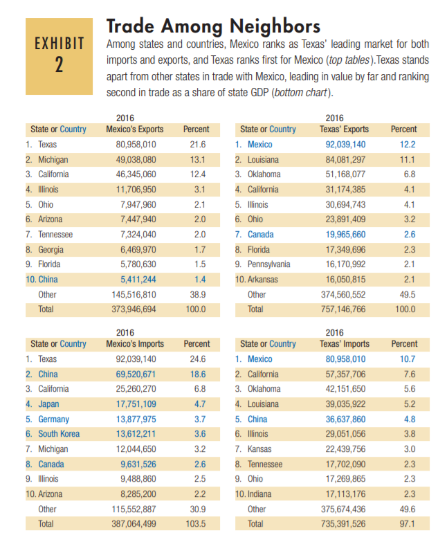
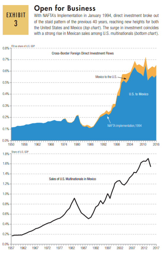
Michael Cox and Richard Alm of SMU’s O’Neil Center have an essay in D Magazine based on the latest report from the Center. The two
imagine Texas and Mexico as one economy, connected by exports, imports, migration, cross-border business investments, transport infrastructure, tourism, and knowledge transfers. As a combined economy, Texas and Mexico churn out an annual GDP of more than $4 trillion, enough to rank as the world’s sixth-largest economy, just behind Germany and ahead of Russia.
We denote this sprawling and diverse economy by the portmanteau word: Texico. The name captures the reality that over the past quarter-century the Texas and Mexico economies have emerged as highly integrated, making an often-unsung contribution to Texas’ reign as America’s top-performing state economy.
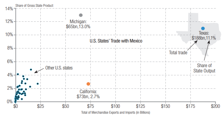
The explain how trade has deeply integrated the two countries:
An often-cited gauge of integration is trade—exports moving south, imports moving north. They totaled $188 billion last year, or more than 11 percent of gross state product, separating Texas from all other states in doing business with Mexico.
Texas companies are finding business opportunities in Mexico—among them, cosmetics-maker Mary Kay Inc. and telecommunications giant AT&T Inc., both based in Dallas-Fort Worth. At the same time, Mexican companies are heading northward and expanding their businesses, including Mission Foods in Irving and the movie theater chain Cinépolis in Addison.
The Texas and Mexico economies are more formidable combined rather than separate. Binational supply chains, for example, take advantage of low production costs in Mexico and highly skilled professional labor in Texas. The companies emerge more competitive in the global marketplace, able to sell their wares at a better price.
Automobile production comes to mind—for good reason. Plants in the Dallas-Fort Worth area are on the northern edge of the Texas-Mexico Automotive SuperCluster region, which includes close to 30 assembly plants and more than 230 parts suppliers in Texas and Mexico’s northern states.
Texas and Mexico have already profited a great deal from their binational economy, even though work began in earnest only recently. Mexico didn’t open its energy and telecom markets until just a few years ago. During negotiations that led to the North American Free Trade Agreement, Mexico clung to its monopolies in these industries. With its oil output falling, Mexico finally lifted its ban on foreign oil and gas companies three years ago. If all goes well, this should be a bonanza for Texas, with its deep roster of oilfield services and exploration companies. The telecom monopoly expired about the same time—and AT&T rushed in with its wireless service.
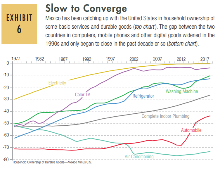
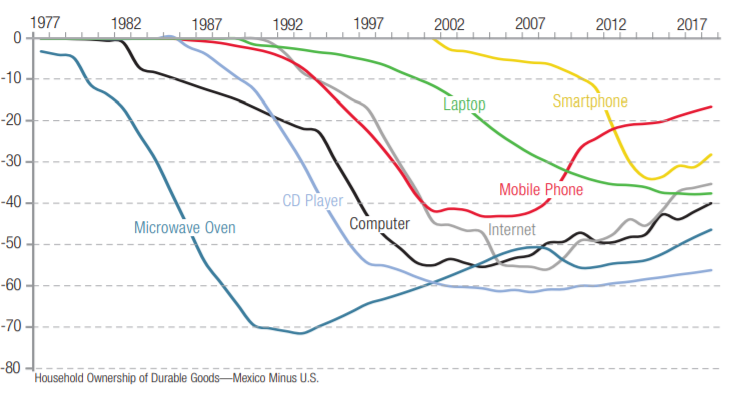
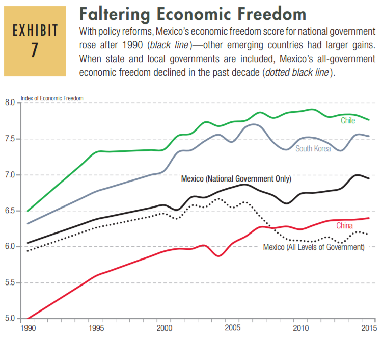
The annual report provides a few more interesting insights:
The report explains the slow convergence above: “Other factors like low levels of education shouldn’t be ignored, but the ongoing plague of corruption, cronyism and rising violence go a long way toward explaining why Mexican growth and income haven’t converged with the United States or kept pace with the likes of Chile, South Korea and China” (pg. 13).
Texans are well aware of Mexico’s shortcomings, including corruption and drug-cartel violence. None of these problems will get any better by enacting policies that build barriers against Mexico and harm the Texas and Mexico economies. Perhaps Trump and Obrador will decide that the best course lies in expedient practicality—recognizing the fact that Texico has been working and building a large constituency. If these two leaders don’t make a mess of things, the businesses of Texas and Mexico can take it from there.
A brand new job market paper has some interesting data on assortative mating and its impact on income inequality. Drawing on data from the Panel Study of Income Dynamics (PSID), the paper
investigates the evolution of assortative mating based on permanent wage in the U.S. since the late 1960s; quantifies its impact on rising family-wage inequality; and, finally, tries to understand the factors behind this evolution. It documents a significant increase in assortative mating, as measured by couple’s permanent-wage correlation, between families formed in the late 1960s and in the late 1980s. I then show that changes in the degree of assortative mating accounts for a sizable amount of the increase in family wage inequality across these family cohorts. This finding shows focusing on the time trends in permanent-wage inequality is not enough to understand the mechanics of increasing family wage inequality. Note, this finding does not rule out a feedback mechanism. It might be that increasing family wage inequality incentivized individuals to care more about their spouse’s wages, causing a higher degree of marital sorting along permanent wage, which in turn mechanically increased family wage inequality (pg. 23).
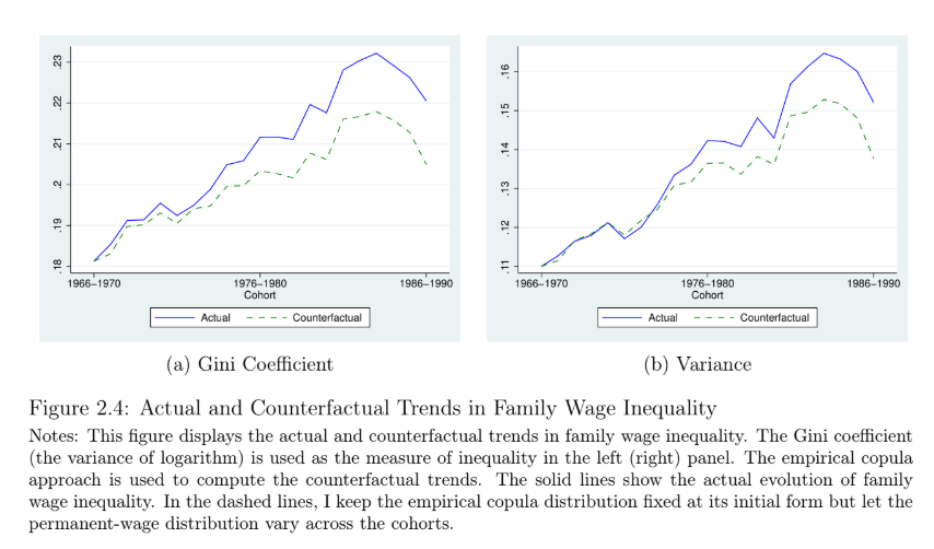
What is “a sizable amount”? The data show that “the trend in assortative mating explains more than one-third of the increase in family wage inequality” (pg. 11; emphasis mine). He explains,
I use the Gini coefficient in the left panel, as the measure of inequality, whereas the variance of logarithm is used in the right panel. Solid lines show the actual evolution of family wage inequality with these measures. In the dashed lines, however, I construct the counterfactual family wage inequality by holding the empirical copula distribution fixed at its initial form while letting the permanent-wage distribution vary. The dashed lines thus show the counterfactual evolution of family wage inequality if no change occurred in assortative mating. The left panel shows the rise in the Gini coefficient would be 40% lower, and the right panel shows that the rise in the variance of (log) family wage would be around 35% lower under the counterfactual scenario. The increase in assortative mating thus accounts for a significant amount of the increase in family wage inequality (pg. 11).
Sociologist W. Bradford Wilcox and economist Joseph Price have an important chapter in a recent Cambridge-published book on the link between family structure and economic growth. They write,
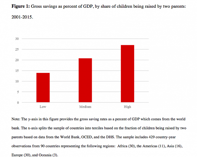
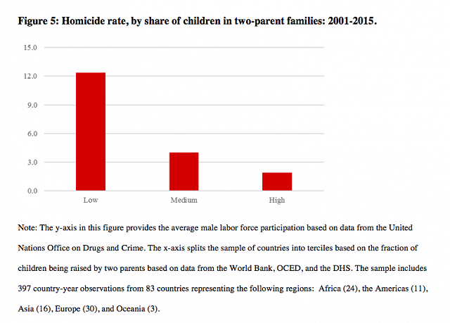
A stable marriage matters in part because it allows couples to make decisions over time that maximize the economic prosperity of their family unit. Stably married persons have incentives to invest in their marriage and benefit from specialization and economies of scale; their households also tend to earn and save more than their peers who are unmarried or divorced (Stevenson and Wolfers 2007; Lerman and Wilcox 2014). Marriage also has a transformative effect on individuals, especially men. It seems to increase men’s productivity at and attachment toward work, and reduces men’s willingness to engage in risky behaviors, including criminal activity (Akerlof 1998; Nock 1998; Sampson, Laub, and Wimer 2006). What is more, it looks like married parenthood may be especially influential in encouraging men’s engagement in the labor force (Killewald 2012). In the aggregate, then, higher levels of marriage, and probably two-parent families, should boost men’s labor force participation and reduce criminal violence, both to the benefit of national economies. At the same time, insofar as motherhood tends to reduce women’s participation in the labor force (Budig and England 2001), we also explore the possibility that higher rates of marriage and two-parent families reduce growth. Finally, higher rates of intact marriage foster stable two-parent families, which are more likely than single parents to supply children with the human capital they need to thrive first in school and later in the labor force (Lerman and Wilcox 2014; McLanahan and Sandefur 1994). Accordingly, the more children are born and raised in stable, two-parent families, the more a society should experience economic growth (pg. 179-180).
Wilcox and Price continue to lay out the evidence that married, two-parents households:
Have more income and savings.
Lower crime rates.
Higher educational achievements for children.
They conclude,
[W]e find that a significant association between family structure and economic growth. Every 13 percentage point increase in the proportion of adults who are married is associated with an 8 percent increase in per capita GDP, net of controls for a range of sociodemographic factors. Likewise, every 13 percentage point increase in the proportion of children living in two-parent families is associated with a 16 percent increase in per capita GDP, controlling for education, urbanization, age, population size, and other factors. There is clearly a link between family structure and economic growth.
…[W]e also note that the cross-national relationship between family structure, household savings, and crime are generally consistent with our expectations about how marriage and two-parent families foster a social environment more conducive to economic growth in countries around the world. It is striking that more two-parent families are linked to less crime and more savings. If nothing else, the patterns documented in this paper suggest that stronger families, higher household savings rates, less crime, and higher economic growth may cluster together in mutually reinforcing ways.
...In conclusion, this chapter indicates that strong and stable families are linked to higher levels of economic growth in nations across the globe, despite the fact that marriage and two-parent families are in decline across much of the globe. Given the potential economic importance of marriage and family stability to a nation’s economic life, policymakers, business leaders, and civic leaders should pursue a range of public and private policies to encourage and strengthen marriage and stable families. That is because what happens in the family may not affect only the welfare of private families but also the wealth of nations (pg. 194-195).
Economic institutions at the macro-level matter. But so do the ones at the micro-level. Probably more so.
As the elections were coming up, I noticed that many wanted to inflate their single vote with undeserved moral capital. I wasn’t having any of it, especially if they were doing so in order to smugly lecture others.
There is some debate among economists and political scientists over the precise way to calculate the probability that a vote will be decisive. Nevertheless, they generally agree that the probability that the modal individual voter in a typical election will break a tie is small, so small that the expected benefit (i.e., p[V(D)−V(R)]p[V(D)−V(R)]) of the modal vote for a good candidate is worth far less than a millionth of a penny (G. Brennan and Lomasky 1993: 56–7, 119). The most optimistic estimate in the literature claims that in a presidential election, an American voter could have as high as a 1 in 10 million chance of breaking a tie, but only if that voter lives in one of three or four “swing states,” and only if she votes for a major-party candidate (Edlin, Gelman, and Kaplan 2007). Thus, on both of these popular models, for most voters in most elections, voting for the purpose of trying to change the outcome is irrational. The expected costs exceed the expected benefits by many orders of magnitude.
While a 1-in-10 million chance is the most optimistic estimate, the average estimate is 1-in-60 million. Economist Steve Landsburg put it this way: “I have a better chance of winning the Powerball jackpot 7,400 times in a row than of affecting the election’s outcome. Which makes it pretty hard to see why I should vote.”[ref]There’s always the comeback, “If everyone thought that, it’d be a disaster!!” Well, not everyone does, so that’s irrelevant. If everyone decided they didn’t want to be a doctor, that’d be a disaster too. Yet, no one says we all have a moral duty to be a doctor. We’re talking about the meaning of your single vote, not the collective’s.[/ref]
So maybe the presidential election is a long shot when it comes to making a difference as an individual voter. Surely the midterm elections are different, right? They certainly are, but it’s not something to get excited about. As economist Casey Mulligan explains,
An election of a United States senator, or a governor, has never in the history of the United States been decided by one vote. Charles Hunter, who earned a doctorate at the University of Chicago, and I studied almost 100 years of elections of members of Congress – almost 20,000 of them in which an aggregate two billion votes were cast – and only one election was determined by a single vote of the 40,000 cast (that was in the New York’s 36th Congressional District in 1910). And that election had a recount that determined the election was decided by a margin of six votes, rather than one.
Thus, when it comes to elections to federal office, history suggests that the chances that your vote…will change the winner of the election is less than one in 100,000; more people die in an election year in car crashes than cast a pivotal vote in a federal election.
Dr. Hunter and I also studied 21 years of elections to state legislatures in the 50 states. Our data included more than 50,000 elections with an aggregate of about a billion votes cast. Those elections were markedly smaller than the federal elections and therefore more likely to come down to one vote.
Still, only nine of these came down to one vote (before recounts), and included a grand total of less than 40,000 pivotal votes. So the probability of a pivotal vote in these elections was less than one in 25,000. (The odds are somewhat higher – one in 15,000 for the state elections and one in 89,000 for Congressional elections – if the election actually has more than one candidate; a number of elections do not, such as this year’s election in Florida’s 21st Congressional District).
Let’s check those stats again:
Presidential elections: 1-in-60 million on average; 1-in-10 million at best.
Federal elections: 1-in-100,000; 1-in-89,000 for Congressional elections.
State legislators elections: 1-in-25,000; 1-in-15,000 at best.
As one friend put it, if you’re trying to get into the Good Place, voting likely earns you 10 points total.[ref]I think that’s rather high, but let’s roll with it.[/ref] That’s a blip on the moral scale.
However, these 10 points are probably cancelled out by:
The smugness that accompanies your “I Voted” sticker.
The likelihood that your Facebook status about the importance of voting is nothing more than moral grandstanding.[ref]”And when thou prayest, thou shalt not be as the hypocrites are: for they love to pray standing the synagogues and in the corners of the streets, that they may be seen of men. Verily I say unto you, They have their reward” (Matt. 6:5). Just replace “pray” with “vote” and the synagogues and street corners with Facebook and Twitter.[/ref]
But that’s still working off the assumption that voting is an inherent good. No one seems to care that voting imposes costs on others by means of legalized violence (government). Now, those costs and the accompanying legalized violence may be justified. But if you’re going to force something on to others, you’d better be damned sure it is in fact just and worth the cost. If you’re not sure (and the social sciencesuggests you probably aren’t), stay away from the polls.
Also, voters typically want to transmit all the goodness of their political picks to themselves, while ignoring the evil. For example, many Obama supporters probably see themselves as champions of the uninsured; crusaders for healthcare justice. However, they likely do not want his drone strikes or deportations on their conscience. “Turns out I’m really good at killing people” isn’t exactly the moral motto most voters want to trumpet.
Finally, you may be risking more harm than good by simply driving to the polls on election day:
[S]uppose my favored candidate (who is worth $33 billion more to the common good) enjoys a slight lead in the polls. She has a very small anticipated proportional majority. The probability that any random voter will vote for her is 50.5 percent. This is an election we would describe as “too close to call.” Suppose also that the number of voters will be the same as in the 2004 U.S. presidential election: 122,293,332. I vote for my favored candidate. In this case, the expected value (for the common good) of my vote for the better candidate is $4.77 x 10^-2650 , that is, approximately zero. Even if the candidate were worth $33 billion to me personally, the expected value for me of my vote would be, again, a mere $4.77 x 10^-2650 . That is 2,648 orders of magnitude less than a penny. In comparison, the nucleus of an atom, in meters, is about 15 orders of magnitude shorter than I am. In meters, I am about 26 orders of magnitude shorter than the diameter of the visible universe. In pounds, I am about 28 orders of magnitude less heavy than the sun. Even if the value of my favored candidate to me were dramatically higher, say ten thousand million trillion dollars, the expected value of my vote in our example—for a close election—remains thousands of orders of magnitude below a penny. For an election in which the candidate has a sizable lead, the expected utility of an individual vote for a good candidate drops to almost zero.
The Beneficence Argument appeals to the public utility of individual acts of voting. However, suppose all you care about is maximizing your contribution to the common good. If so, voting would not merely fail to be worthwhile— it would be counterproductive. It turns out that the expected disutility of driving to the polling station (in terms of the harm a driver might cause to others) is higher than the expected utility of a good vote. This is not hyperbole.
Aaron Edlin and Pinar Karaca-Mandic have estimated the expected accident externalities per driver per year in the United States—that is, the amount of damage the average driver imposes on others from accidents and reckless driving. The expected accident externalities range from as little as $10 in low-traffic-density North Dakota to more than $1,725 in high-traffic-density California. Suppose a North Dakotan takes five minutes to drive to the polling station. The average expected accident externality of a five-minute drive in North Dakota is $9.5 x 10^-5 , much larger than the expected benefit of a good vote in the previous example. So the voter imposes greater expected harm on her way to the polls than she could compensate for by a good vote.[ref]Jason Brennan, The Ethics of Voting, pg. 19-20.[/ref]
To review:
Mathematically speaking, your individual vote has probably never mattered and likely never will matter. It literally has no consequence on the planet.
Whatever goodness your single vote represents is likely cancelled out by a number of negative factors that are the byproduct of political participation.
In actuality, voting is a means of wielding legalized violence on others.
If you’re going to congratulate yourself on the good your chosen politician does, you have to condemn yourself for the bad as well.
The risk of harming others on election day is higher than the potential benefit.
Now, this isn’t an anti-voting post. I’m not saying you should refrain from voting.[ref]Unless you don’t know jack about what or who you’re voting for. In that case, stay home. I actually think you’re a better person for doing so.[/ref] What I am saying is that before you start patting yourself on the back for supposedly righting the wrongs of the world through voting, you ought to realize that you probably did absolutely nothing.
It’s a common assertion by some people that the rich are obviously awful people. Some psychology research (especially that of Paul Piff) seems to confirm that wealth makes us worse people. However, a new study casts doubt on some of these findings, demonstrating that the field of psychology is still having replication problems. “In contrast [to Piff’s work],” write the authors,
The authors “attempted to directly replicate Piff et al.’s Study 5 (2012),” which tested individuals’ willingness to lie in a negotiation task.
In an effort to increase experimental power, the present studies sought to increase sample size from 108 to 270 (i.e., 2.5 times larger), which is considered the current standard for replication protocols (Simonsohn, 2015). We collected two independent samples in an effort to provide more opportunity to replicate the original results (e.g., larger number of participants across samples helps mitigate issues associated with sampling error).
Their results?
Some of our findings were consistent with those of Piff et al., such as the significant relations between attitudes toward greed and unethical behaviour (i.e., dishonesty) as well as between social class and greed (in sample 2 only), but we did not obtain any evidence of a positive association between social class and unethical behaviour in either sample. Further, we found inconclusive evidence for the mediation model proposed by Piff et al. across the two samples.
Perhaps the crucifixion of the rich isn’t the most empirically-based idea.